14 Hypothesis Testing and Standard Error
In this chapter, we’ll develop a comprehensive understanding of hypothesis testing through a detailed worked example. We’ll build the theoretical foundation step by step, introducing key concepts like standard error, test statistics, and p-values along the way. By the end of this chapter, you will understand how to conduct hypothesis tests for population means, interpret their results, and recognize the crucial differences between large and small sample tests.

14.1 The Problem: Evaluating a New Curriculum
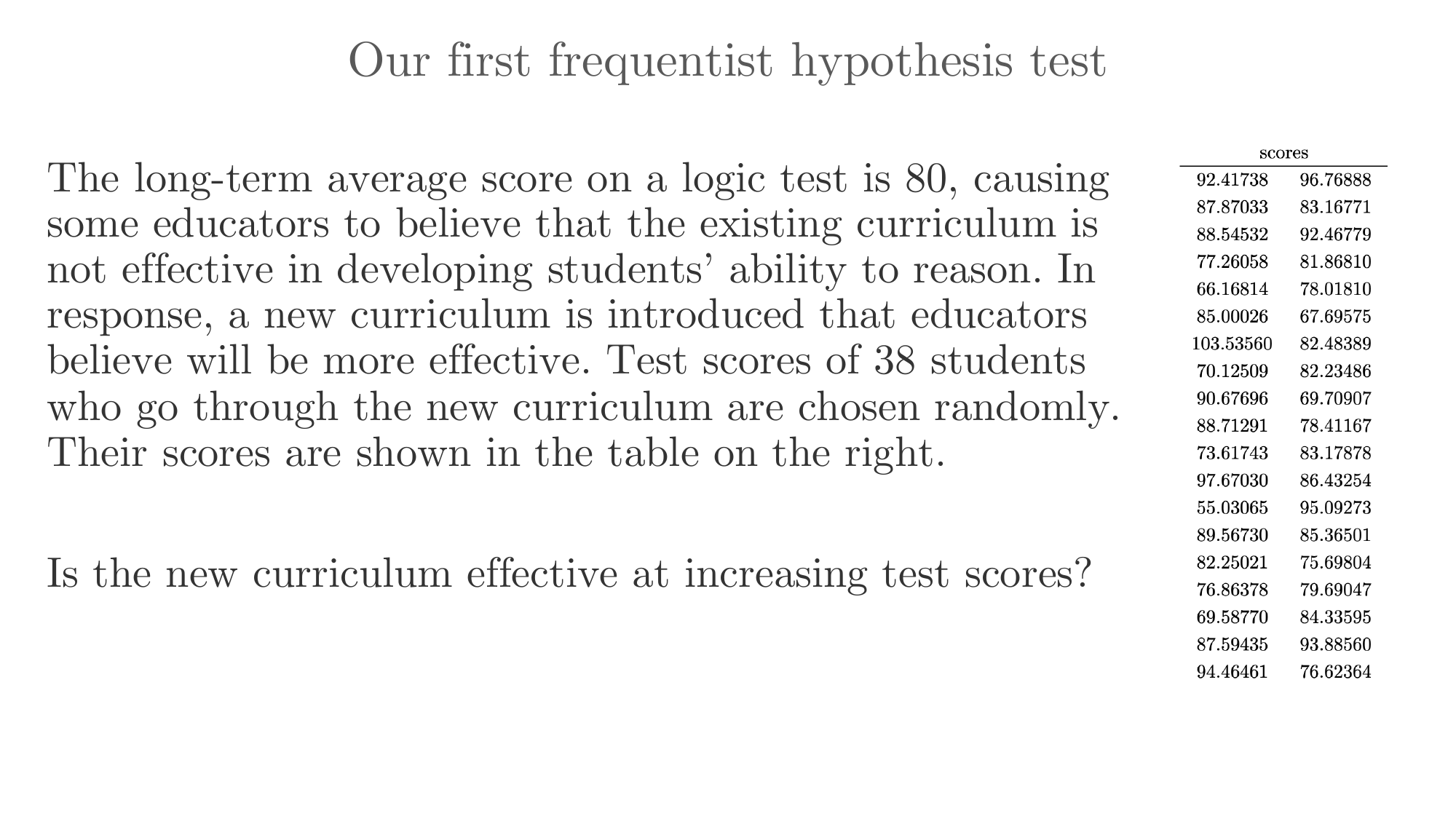
Let’s begin with a concrete problem that will guide our exploration of hypothesis testing. Suppose we’re trying to improve the logical ability of students through a new curriculum. The old curriculum, which has been in use for many years, produces an average test score of 80 points. We’ve developed a new curriculum and trained a large group of students using this approach.
The central question we want to answer is: Is the new curriculum more effective at raising average test scores?
To investigate this question, we randomly sample 38 students from those trained under the new curriculum and record their test scores. Our sample yields a mean score of 83 points.
The Logic of Hypothesis Testing
Frequentist hypothesis testing operates on a principle analogous to proof by contradiction in mathematics. We temporarily assume the opposite of what we hope to demonstrate, then show that this assumption leads to implausible results.

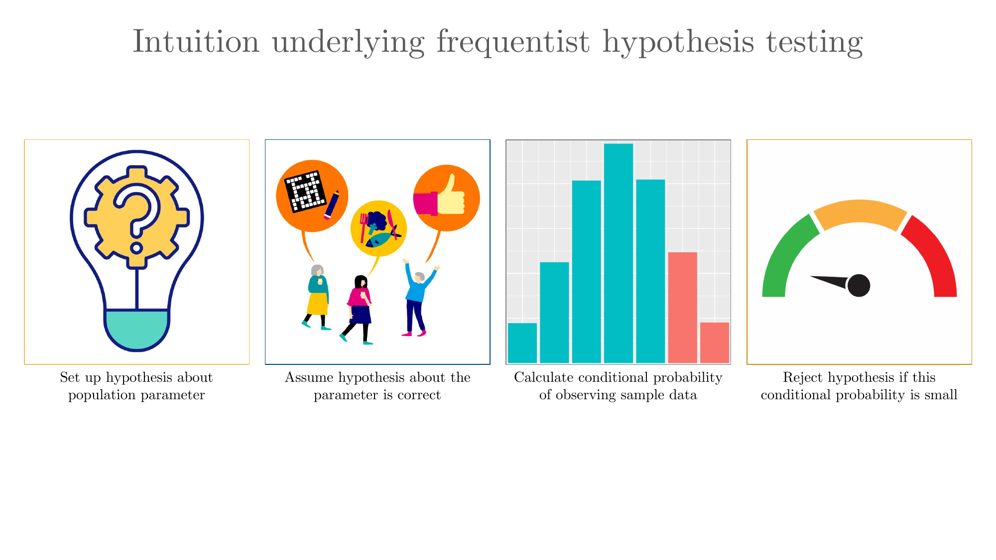
The intuition is straightforward: we set up a hypothesis about a population parameter, assume it’s correct, then calculate the conditional probability of observing our sample data. If this probability is sufficiently small, we reject the hypothesis.
14.2 Understanding Standard Error
Before we can conduct a proper hypothesis test, we need to understand a crucial concept: standard error.
The Concept of Repeated Sampling
To truly understand standard error, we need to embrace a core principle of frequentist statistics: repeated sampling. Imagine we could draw not just one sample of 38 students, but millions of such samples from our population. Each sample would give us a different sample mean.
Here’s the remarkable thing: if we computed all these sample means and calculated their average, that average would equal the true population mean. This property is called unbiasedness, and it’s why we use the sample mean as our estimator.
But these individual sample means would vary around the population mean. The standard error tells us the typical size of this variation. In our example, with a sample size of 38 and a calculated standard error of 1.64 points, we know that a typical sample mean deviates from the population mean by about 1.64 points.
The Relationship: Population Variance to Sample Mean Variance
There’s a fundamental relationship connecting the population variance to the variance of the sample mean:
\[ \text{Var}(\bar{Y}) = \frac{\sigma^2}{n} \]
Taking the square root of both sides gives us the standard error formula. This relationship tells us that:
- The variance of sample means is smaller than the population variance
- This variance decreases as sample size increases
- The relationship is inverse with sample size (doubling \(n\) doesn’t double precision)
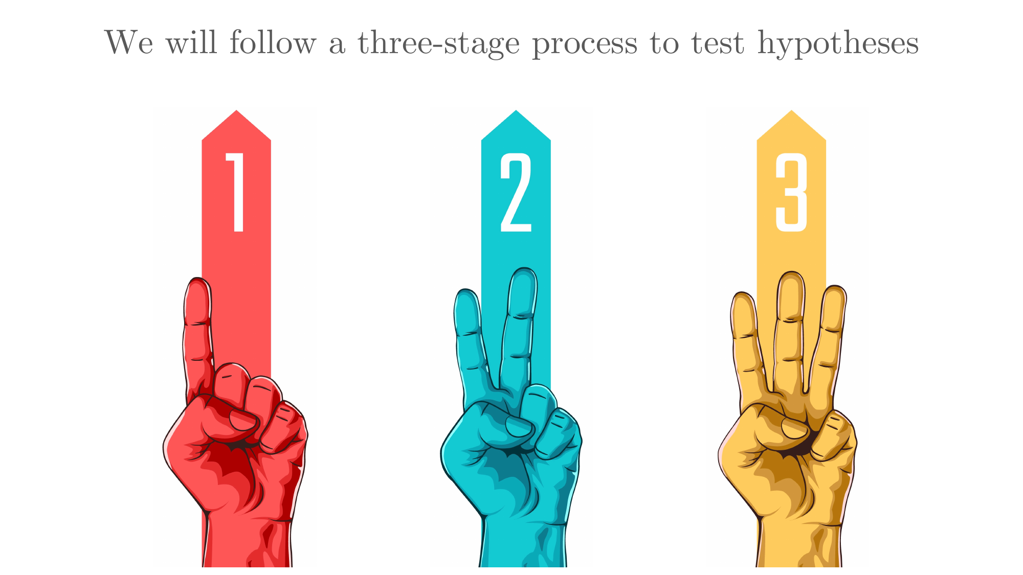
14.3 The Three Stages of Hypothesis Testing
Now that we understand standard error, we can proceed with our hypothesis test. We’ll work through this systematically in three stages.
Stage 1: Formulating the Hypotheses
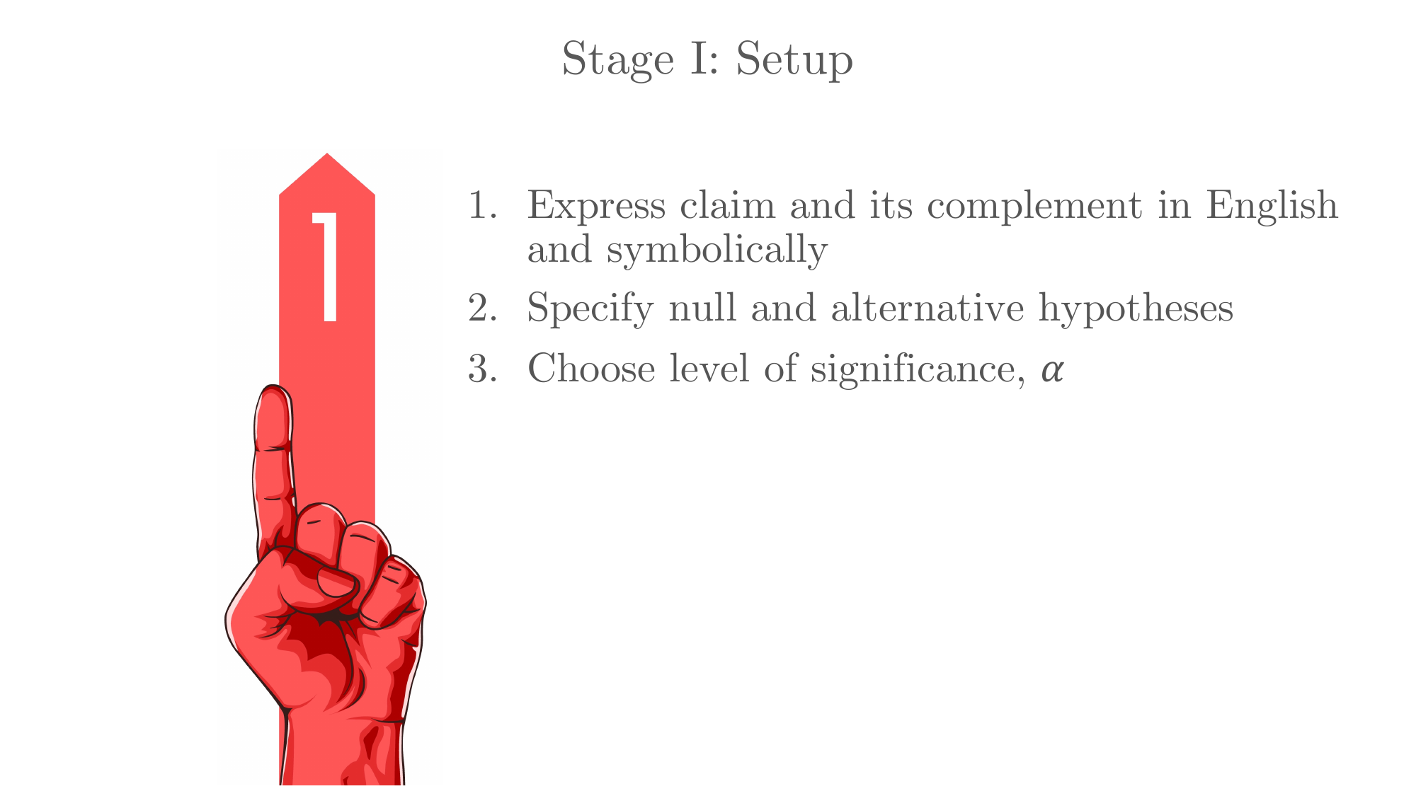
The first step in any hypothesis test is to clearly state what we’re testing. We need two competing hypotheses.
Expressing Our Claim in English
Claim: Students trained under the new curriculum will score, on average, higher than 80 on the test.
Complement: Students trained under the new curriculum will not score, on average, higher than 80 on the test.
The Law of the Excluded Middle
In formulating our hypotheses, we’re invoking a fundamental principle of logic: the law of the excluded middle.
This law states that a statement is either true or false—there is no middle ground between truth and falsity. Either the new curriculum improves scores beyond 80, or it doesn’t. Our job is to determine which is more likely given our data.
Symbolic Representation
Let the mean score of students trained under the new curriculum be \(\mu\).
Claim: \(\mu > 80\)
Complement: \(\mu \leq 80\)
Assigning Null and Alternative Hypotheses
Null Hypothesis (\(H_0\)): The population mean test score under the new curriculum is less than or equal to 80. \[ H_0: \mu \leq 80 \]
Alternative Hypothesis (\(H_A\)): The population mean test score under the new curriculum exceeds 80. \[ H_A: \mu > 80 \]
The null hypothesis represents the status quo or the claim we’re trying to find evidence against. The alternative hypothesis represents what we hope to demonstrate with our data. By convention, we assign the complement of our claim to the null hypothesis—this is what we will attempt to falsify.
We also need to choose a significance level \(\alpha\), which represents our tolerance for making a Type I error (rejecting a true null hypothesis). Let’s set \(\alpha = 0.04\) or 4%.
Understanding Type I and Type II Errors
Before proceeding, we must acknowledge that hypothesis testing involves the possibility of error. There are two types of errors we might make:
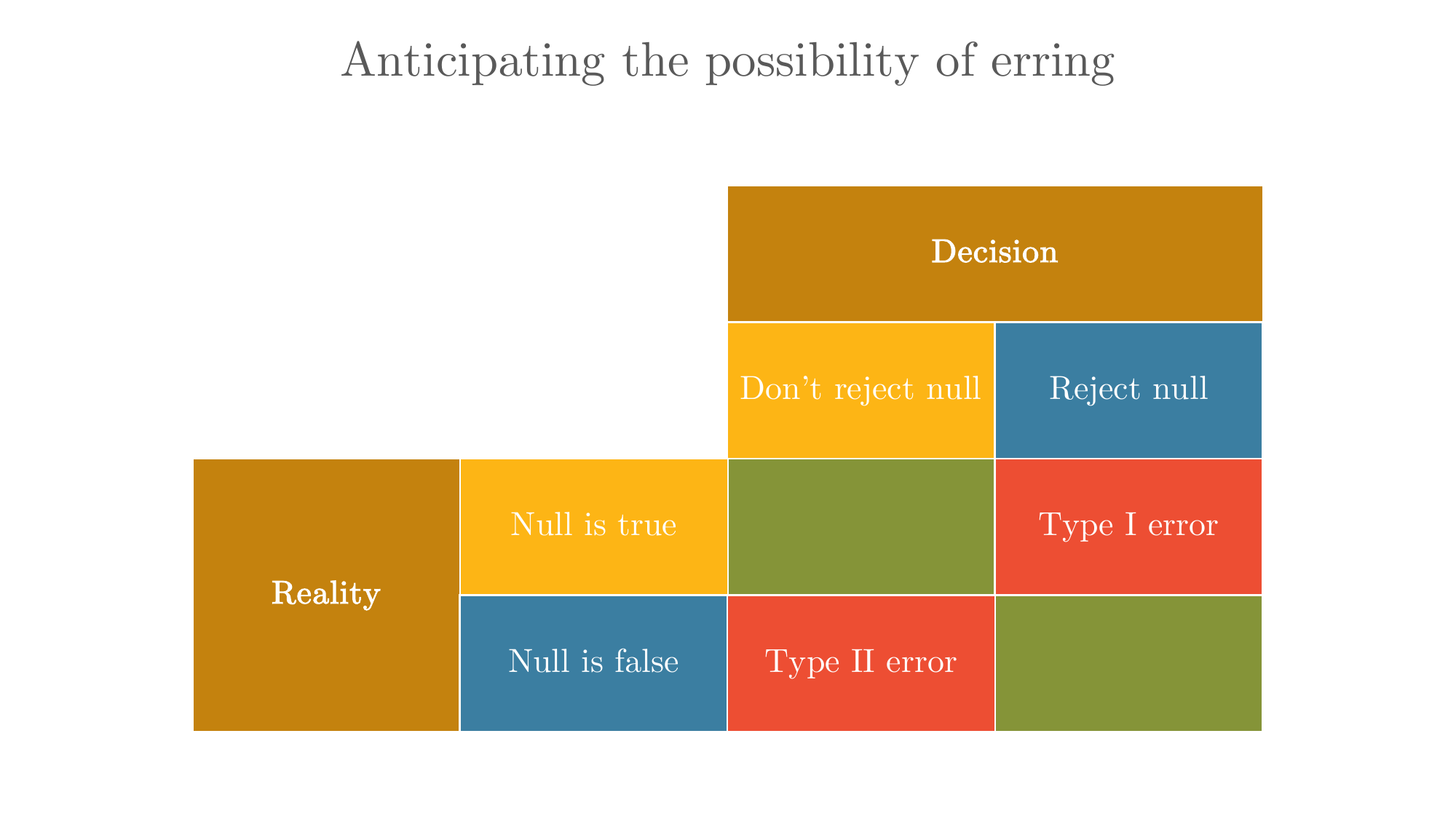
Type I Error: Rejecting a true null hypothesis (false positive) Type II Error: Failing to reject a false null hypothesis (false negative)
It’s crucial to understand that we cannot make both errors simultaneously:

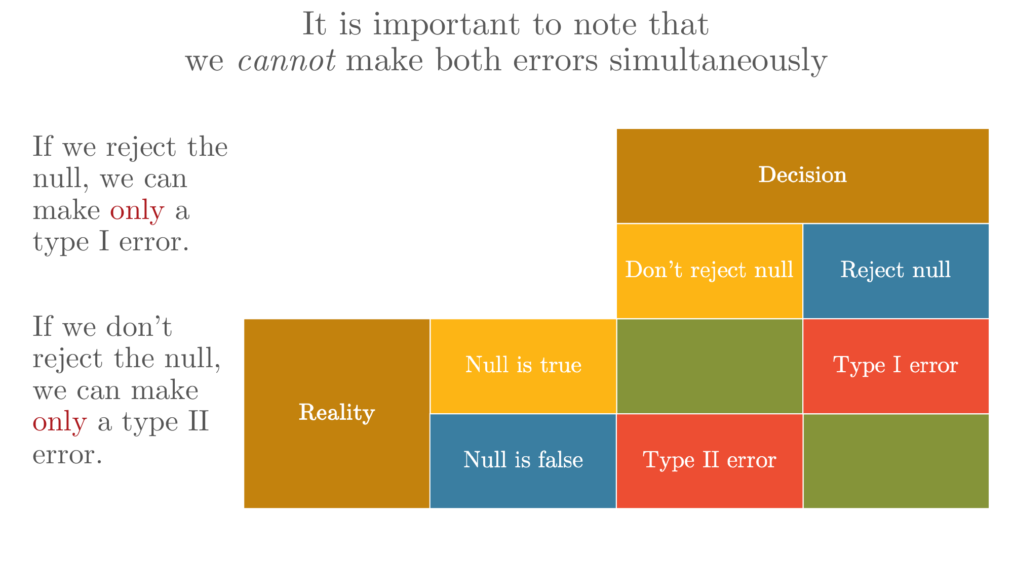
- If we reject the null, we can make only a Type I error
- If we don’t reject the null, we can make only a Type II error
Choosing the Significance Level
We also need to choose a significance level \(\alpha\), which represents our tolerance for making a Type I error (rejecting a true null hypothesis).

In many academic papers, the level of significance is set at either 5% or 1%. But where do these specific values come from?

The answer involves both history and convention. The story begins with an afternoon tea party and R.A. Fischer.
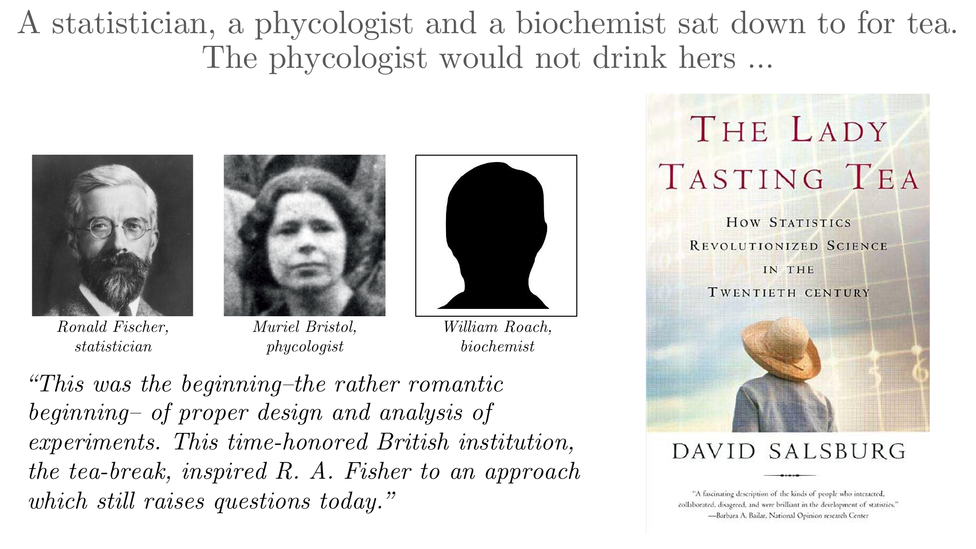
Fischer’s work on experimental design, inspired by a colleague who claimed she could tell whether milk was added before or after tea, led to the development of significance testing as we know it today.
Stage 2: Estimating the Sampling Distribution
In this stage, we need to characterize the distribution of our test statistic under the assumption that the null hypothesis is true.
Step 1: Choose an Estimator
We use the sample mean \(\bar{Y}\) as our estimator of the population mean \(\mu\). Our observed value is \(\bar{y} = 83\).
Step 2: Establish the Distribution
The sample mean is itself a random variable. With our large sample size (\(n = 38\)), we can invoke the Central Limit Theorem (CLT), which tells us that the sampling distribution of \(\bar{Y}\) is approximately normal, regardless of the shape of the population distribution.
\[ \bar{Y} \sim N(\mu, \sigma^2/n) \]
Step 3: Estimate the Parameters
Under the null hypothesis, we assume \(\mu \leq 80\). For the purposes of constructing our test, we’ll use \(\mu = 80\) as the boundary value (the null hypothesis “at its most extreme”).
From our sample data, we calculate: - Sample standard deviation: \(s = 10.1\) points - Standard error: \(SE = s/\sqrt{n} = 10.1/\sqrt{38} \approx 1.64\) points
Visualizing the Distribution
Imagine a bell curve centered at 80. This represents all possible sample means we could observe if the true population mean were 80. Some sample means would be less than 80, some greater, but they’d cluster around 80 with most values falling within a few standard errors of the center.
Our observed sample mean of 83 lies to the right of this center. The question is: is it far enough to the right that we should doubt the null hypothesis?
Stage 3: Computing the Test Statistic and P-value
To answer our question, we need to standardize our observed value and determine how unusual it is.
The Test Statistic: Zeta (ζ)
We define a test statistic called zeta (ζ) as:
\[ \zeta = \frac{\bar{Y} - \mu_0}{SE} \]
where \(\mu_0\) is the hypothesized population mean under the null (80 in our case).
This standardization accomplishes two things: 1. It converts our result to a unit-free measure 2. It tells us how many standard errors our observed mean is from the hypothesized mean
Calculating Our Test Statistic
For our problem: \[ \zeta = \frac{83 - 80}{1.64} = \frac{3}{1.64} \approx 1.83 \]
Our observed sample mean is 1.83 standard errors above the hypothesized mean of 80.
The Distribution of Zeta
When the sample size is large and we know (or can estimate) the population standard deviation, the test statistic ζ follows a standard normal distribution (also called a Z-distribution). This is the same as the Z-scores you may have encountered before.
\[ \zeta \sim N(0, 1) \]
Computing the P-value
The p-value answers the question: “If the null hypothesis were true, what is the probability of observing a test statistic as extreme as or more extreme than what we actually observed?”
For our one-sided test: \[ p\text{-value} = P(\zeta \geq 1.83 \mid H_0 \text{ is true}) \]
Using a standard normal table or software, we find: \[ p\text{-value} \approx 0.034 \text{ or } 3.4\% \]
Making the Decision
We compare our p-value to our significance level: - p-value = 3.4% - \(\alpha\) = 4%
Since the p-value (3.4%) is less than our significance level (4%), we reject the null hypothesis.
14.4 Visual Interpretation
Let’s visualize what we’ve done. Picture the sampling distribution under the null hypothesis: a normal curve centered at 80 with standard deviation 1.64. Our observed sample mean of 83 falls in the right tail of this distribution.
The p-value is the area under this curve to the right of 83—it represents how much of the distribution lies at or beyond our observed value. This area is relatively small (3.4%), indicating that our observation would be quite unusual if the null hypothesis were true.
14.5 The Small Sample Case: When n < 30
Everything we’ve done so far assumes a large sample (typically \(n \geq 30\)). But what happens when we have a small sample? The mathematics changes in an important way.
The Problem with Small Samples
Consider the same problem, but now suppose we only have \(n = 24\) students in our sample. The sample mean is still 83, and the sample standard deviation is still 10.1.
The key difference: when we use the sample standard deviation \(s\) to estimate the population standard deviation \(\sigma\), we introduce additional uncertainty. This uncertainty becomes problematic when the sample size is small.
William Gosset’s T-Distribution
In the early 1900s, William Sealy Gosset (writing under the pseudonym “Student” because his employer, Guinness Brewery, didn’t allow employees to publish) discovered that for small samples, the test statistic doesn’t follow a normal distribution—it follows a t-distribution.
The test statistic is still calculated the same way: \[ \zeta = \frac{\bar{Y} - \mu_0}{s/\sqrt{n}} \]
But now, instead of following a Z-distribution, ζ follows a t-distribution with \(\nu = n-1\) degrees of freedom: \[ \zeta \sim t_{\nu} \]
Properties of the T-Distribution
The t-distribution looks similar to the normal distribution—it’s symmetric and bell-shaped—but it has heavier tails. This reflects the additional uncertainty from estimating the standard deviation.
Key properties: 1. As the degrees of freedom increase, the t-distribution approaches the normal distribution 2. For small degrees of freedom, the tails are much heavier than the normal 3. By \(\nu \approx 30\), the t-distribution is virtually indistinguishable from the normal
Comparing the Two Ratios
Let’s clarify the distinction between two similar-looking ratios:
Ratio A (with known σ): \[ \text{Andrew} = \frac{\bar{Y} - \mu_0}{\sigma/\sqrt{n}} \]
Ratio B (with estimated s): \[ \text{Ben} = \frac{\bar{Y} - \mu_0}{s/\sqrt{n}} \]
Small Sample Analysis: Our Example
Let’s return to our curriculum problem with the small sample of 24 students:
- \(n = 24\)
- \(\bar{y} = 83\)
- \(s = 10.1\)
- \(SE = 10.1/\sqrt{24} \approx 2.06\)
Test statistic: \[ \zeta = \frac{83 - 80}{2.06} \approx 1.46 \]
This time, ζ follows a t-distribution with 23 degrees of freedom. Looking up this value in a t-table or using software:
\[ p\text{-value} \approx 0.08 \text{ or } 8\% \]
The Decision Changes
Now our p-value (8%) exceeds our significance level (4%). We fail to reject the null hypothesis.
When to Use Each Distribution
Use the Z-distribution (normal) when: - Sample size is large (\(n \geq 30\)) - Population standard deviation σ is known (rare in practice)
Use the t-distribution when: - Sample size is small (\(n < 30\)) - Population standard deviation σ is unknown and must be estimated from the sample
In practice, many statisticians use the t-distribution for all tests involving estimated standard deviations, regardless of sample size. As the degrees of freedom increase, the t-distribution becomes virtually identical to the normal, so using the t-distribution is a conservative choice that’s always appropriate.
14.6 Summary: The Hypothesis Testing Framework
Let’s review the complete process we’ve developed:
Stage 1: Set Up 1. State the null and alternative hypotheses 2. Choose a significance level α 3. Identify the test type (one-sided or two-sided)
Stage 2: Characterize the Sampling Distribution 1. Select an appropriate estimator 2. Use theory (CLT) to establish its distribution 3. Estimate the parameters of this distribution 4. Visualize the distribution under \(H_0\)
Stage 3: Test and Decide 1. Calculate the test statistic (ζ) 2. Determine its distribution (Z or t) 3. Compute the p-value 4. Compare p-value to α and make a decision 5. State your conclusion in context
14.7 Looking Ahead: Two-Sample Tests and Causality
The hypothesis test we’ve developed compares a population mean to a known constant (80). While this is valuable for understanding the mechanics of hypothesis testing, it’s relatively rare in practice.
More commonly, we want to compare two groups: a control group and a treatment group. This leads to two-sample tests, which will be our next topic.
Two-sample tests look very similar mechanically to what we’ve done here, with a crucial philosophical difference: they allow us to investigate causality. By comparing a treatment group to a control group, we can begin to assess whether an intervention has a causal effect on an outcome.
The foundation you’ve built here—understanding sampling distributions, standard errors, test statistics, and p-values—will carry forward directly to these more powerful tests. The transition is a relatively small mechanical extension, but it opens the door to answering causal questions.